Overview
Promises and pitfalls of using predicted data for downstream inference
Background and Motivation
Artificial intelligence and machine learning (AI/ML) have become essential tools in biomedical research, enabling large-scale analyses across diverse domains such as genomics, structural biology, and electronic health records-based research. Increasingly, researchers rely on model-generated predictions, rather than directly measured variables, as inputs for downstream statistical analyses. For example, predicted gene expression values or polygenic risk scores are often used in place of experimental assays, allowing researchers to expand cohort sizes and explore hypotheses when traditional data collection is infeasible, costly, or time-consuming.
While this practice of “using predictions as data” holds promise for accelerating scientific discovery, it presents significant challenges for statistical inference. When predicted values are used in place of true variables, the resulting estimates of association can be biased and misleading if uncertainty in the prediction step is not properly accounted for.
Modern biomedical analyses increasingly rely on machine learning predictions as inputs to downstream statistical models. This can expand scope and improve feasibility, but treating predictions as if they were observed data can bias effect estimates and understate uncertainty.
Setup
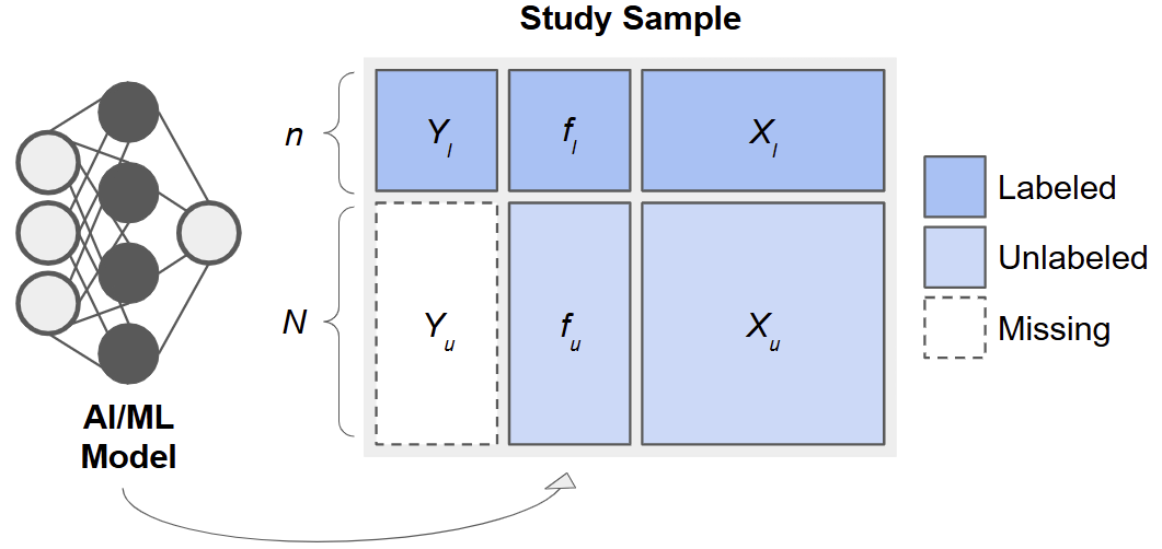
When an outcome, \(Y\), is costly or difficult to measure, it can be tempting to replace missing values with predictions, \(f(\boldsymbol{X})\), from a machine learning model (e.g., a random forest or neural network) built on easier-to-measure features, \(\boldsymbol{X}\). However, using \(f\) as if it were the true outcome in downstream analyses, e.g., in estimating a regression coefficient, \(\beta\), for the association between \(Y\) and \(\boldsymbol{X}\), leads to biased point estimates and underestimated uncertainty. Methods for Prediction-Based (PB) Inference address this by leveraging a small subset of “labeled” data with true \(Y\) values to calibrate inference in a larger “unlabeled” dataset.
The Prediction-Based (PB) Inference Framework
Consider data arising from three sets of observations:
- Training Set: \(\{(X_j, Y_j)\}_{j=1}^{n_t}\), used to fit a predictive model, \(f(\cdot)\).
- Labeled Set: \(\{(X_i, Y_i)\}_{i=1}^{n_l}\), smaller sample with true outcomes measured.
- Unlabeled Set: \(\{(X_i)\}_{i=n_l +1}^{n_l + n_u}\), only features available.
After fitting \(f\) on the training set, we apply it to the labeled and unlabeled sets to obtain predictions \(f_i = f(X_i)\)
Especially for ‘good’ predictions, it is tempting to treat \(f_i\) as surrogate outcomes and use them to estimate quantities such as regression parameters, \(\beta\). However, as we will see, this leads to invalid inference. By combining the predicted \(f_i\) with the observed \(Y_i\) in the labeled set, we can calibrate our estimates and standard errors to achieve valid inference.
Key Formulas
Consider a simple linear regression model for the association between \(Y\) and \(X\). We discuss the following potential estimators, which we will later implement using simulated data.
Naive Estimator
Using only the unlabeled predictions, the naive OLS estimator solves
\[ \hat\gamma_{\text{naive}} = \arg\min_\gamma \sum_{i\in U} (f_i - X_i'\gamma)^2. \]
We are careful to write the coefficients for this model as \(\gamma\), because they bear no necessary correspondence with \(\beta\), except under the extremely restrictive scenario when \(f\) perfectly captures the true regression function.
Classical Estimator
Instead, a valid approach would be to use only the labeled data. This classical estimator solves
\[ \hat\beta_{\text{classical}} = \arg\min_\beta \sum_{i\in L} (Y_i - X_i'\beta)^2. \] While this approach is valid, it has limited precision because \(n_l\) is small in practice and we do not utilize any potential information from the (often much larger) unlabeled data.
PB Estimators
Many estimators tailored to PB inference share a similar form, as given in Ji et al. (2025):
\[ \widehat\beta_\text{pb} = \arg\min_\beta \frac{1}{n_l}\sum_{i=1}^{n_l} \ell(X_i, Y_i) - \left[\frac{1}{n_l}\sum_{i=1}^{n_l} g(X_i, f_i) - \frac{1}{n_l+n_u}\sum_{i=n_l+1}^{n_l+n_u} g(X_i, f_i)\right], \]
for some loss function, \(\ell(\cdot)\), such as the squared error loss for linear regression, and some \(g(\cdot)\), which they call the ‘imputed loss’. Here, the first term is exactly the classical estimator, which anchors these methods on a valid model, and the second term in the square brackets ‘augments’ the estimator with additional information from the predictions. This allows us to have an estimator that is provably unbiased and asymptotically at least as efficient as the classical estimator, which only uses a fraction of the data.
The ipd (inference with predicted data) package implements several recent methods for PB inference, such as the Chen & Chen method of Gronsbell et al., the Prediction-Powered Inference (PPI) and PPI++ methods of Angelopoulos et al. (a) and Angelopoulos et al. (a), the Post-Prediction Inference (PostPI) method of Wang et al., and the Post-Prediction Adaptive Inference (PSPA) method of Miao et al. to conduct valid, efficient inference, even when a large proportion of outcomes are predicted.